1949) Hebbian Learning: The root of Unsupervised Learning

Reference:

https://www.youtube.com/watch?v=7kELUTwjCp8&t=181s

https://en.wikipedia.org/wiki/Hebbian_theory

https://thedecisionlab.com/reference-guide/neuroscience/hebbian-learning/ 

---

Introduction

Timeline

전 포스트에서 설명했듯이, Rosenblatt's Perceptron은 Hebbian theory에 영감을 받아 제안된 아이디어였다. 오늘은 Hebbian Learning에 대해서 알아보겠다.

 

Donald Olding Hebb

“Psychology and Philosophy were divorced some time ago but, like other divorced couples, they still have problems in common” – Donald Hebb in his book, Essays on Mind, 1980.

 

캐나다 출신 선생님이자 심리학자 Hebb는 맥길대학교 석사시절 neural network에 관심을 보였다. 특히 심리-생리학에 관심이 있었던 Hebb은 당대 유명했던 행동주의자(behaviourist) Karl Lashley라는 분과 시카고대학교에서 박사공부를 시작한다. 당시 Hebb은 행동주의와 생리학/신경과학(neuroscience)를 접목한 연구에 집중했다. 후에 Lashley를 따라 하버드 대학교로 가서 1936년 졸업 후 1937년 몬트리올 신경학기관에 돌아와 Wilder Penfield와 일을하게 되는데, Lashley를 포함한 다른 심리학자의 '인지기능(특히 memory와 관련된 기능)이 어떻게 뇌의 특정 부분에 국부화되는가'의 관련된 연구에 영감을 받아 1949년 아직까지도 유명한 그의 책 The Organization of Behaviour에서 Hebbian Learning을 처음 제시한다. 이 이론은 Hebb's rule, Hebb's postulate, 그리고 cell assembly theory 이라고도 불린다.

 

Neurons that fire together, wire together. –Donald Hebb

 

Hebbian Learning은 학습의 심리학적 근거와 신경학적 근거를 연결시키는데에 의의가 있었다. 아이디어의 전반적 설명은 이렇다. 우리가 새로운 것을 배울 때, 우리의 뇌에서는 복잡하게 얽히고 설킨 뉴런들이 fire!하게되고 (전 포스트의 intro 참조) 그 일련의 뉴런집합들이 neural network를 형성하게 된다. 이 연결고리들은 처음에는 약하게 시작되었다가 자극이 반복되면 서서히 강해지며 그 행동이 아주 자연스럽고 본능적이게 변해간다는 것이다. 이 아이디어는 굉장히 직관적이다. 우리가 살면서 공부외에도 많은 행동과 생각들을 하게되는데 많은 시간 반복하면 자신감이 생기는 것이 neural network의 연결이 강해지기 때문이다. 

---

Hebbian Leraning

 

그는 The Organization of Behaviour에 다음과 같이 적었다.

Let us assume that the persistence or repetition of a reverberatory activity (or "trace") tends to induce lasting cellular changes that add to its stability. ... When an axon of cell A is near enough to excite a cell B and repeatedly or persistently takes part in firing it, some growth process or metabolic change takes place in one or both cells such that A’s efficiency, as one of the cells firing B, is increased. 

쉽게 말해, 'Neurons that fire together, wire together.' 라는 뜻이다. 동시에 활성화되는 뉴런들의 weight는 증가하고 따로 활성화되는 뉴런들의 weight는 감소된다. 

Algorithm은 다음과 같이 간략화될 수 있다.

---

Step 1: Initialization

    Set initial synaptic weights and thresholds to small random values in the interval [0,1].

 

Step 2: Activation.

    Compute the postsynaptic neuron output from the presynaptic inputs element $X_{ij}$ in the data-item $X_j$.

 

$\textrm{if} \quad \sum_{i}^{}(X_{ij}Y_{ij})-T\ge 0 :Y_j=1 \quad else \quad Y_j=0$

 

   where $i$ refers to inputs to postsynaptic neuron from presynaptic neurons (쉽게 말해 몇번째 뉴런?), $j$ referes to the training instance considered (쉽게 말해 몇번째 그룹? or 몇번째 iteration?), $T$ is the threshold value of neuron

 

Step 3: Learning - the activity product rule

    Update the weights in the network. The weight correlction is determinded by the activity product rule:

 

$W_{i(j+1)}=W_{ij}+\alpha Y_jX_{ij}$   

 

    where $\alpha$ is the learning rate parameter.

 

Step 4: Iteration

    Go back to step 2

---

Step 3를 보면 알겠지만 weight update의 방식이 Perceptron과 다르다; Perceptron에서는 $w=w+error*x_j=w+(y_j-\sigma (w^Tx_j+b))*x_j$ 방식으로 update를 한다.

아래와 같은 예시를 생각해보자.

2개의 training dataset

1 0 1 0

1 0 1 0

이 있다고 가정.

 

First iteration

 

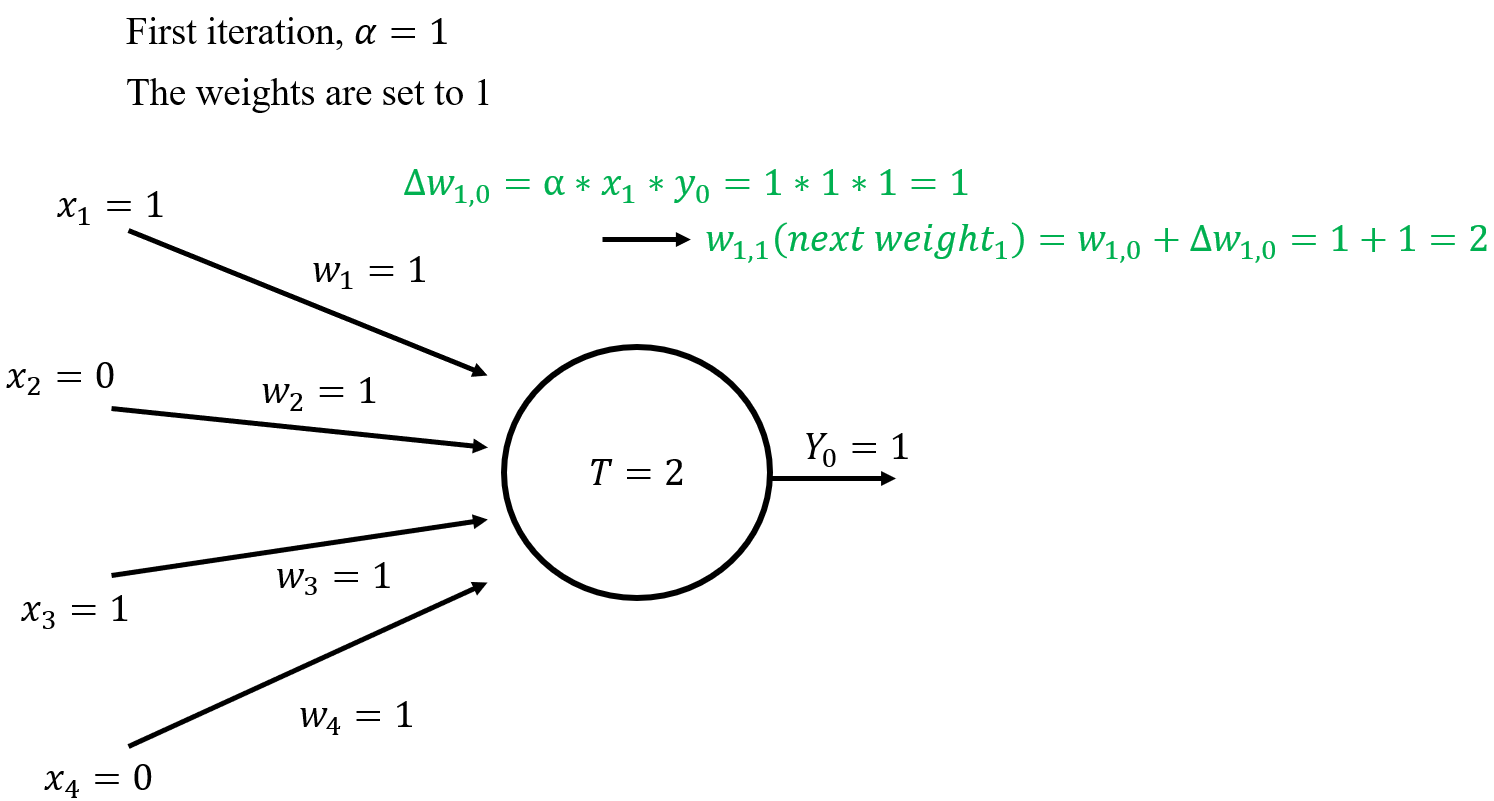
$\textrm{Sum}=\sum_{i=1}^{4}x_iw_i=1*1+0*1+1*1+0*1-2=0\geq 0$ 

$\therefore Y_0=0$

$\Delta w_1=\alpha*x_1*y_0=1*1*1=1$

같은 방식으로, $\Delta w_2=0,\quad \Delta w_3=1,\quad \Delta w_4=0$

이로부터 $w_{1,1}=w_{1,0}+\Delta w_{1,0}=1+1=2$

같은 방식으로, $w_{2,1}=1,\quad w_{3,1}=2,\quad w_{4,1}=1$

 

첫 iteration이 끝나고 얻어진 updated weight로 다음 iteration은

 

Second iteration

 

$\Delta w_1=1, \quad \Delta w_2=0, \quad \Delta w_3=1, \quad \Delta w_4=0$

$w_{1,2}=3, \quad w_{2,2}=1, \quad w_{3,2}=3,\quad w_{4,2}=1$

 

Stimuli: $x_1, x_2$들에 의해 weight가 계속 크게 업데이트 되어 connection이 강화된다는 Hebbian learning의 아이디어를 확인할 수 있다.